
ロンドン大学で MSc Computer Science: Fundamentals of computing モジュールを履修中。
講義内容に関して記録した個人的なスタディノートです。
全 12 週のうち 6〜12 週目の内容を記録します。(6 週目開始:2025 年 2 月 10 日 / 12 週目終了:2025 年 3 月 31 日)
Week 6: Finite state machines #
キーコンセプト
This topic includes:
- regular languages
- alphabets
- finite state machines
- deterministic finite state machines.
レクチャーリスト
- Introduction to regular languages and alphabets
- Lecture 1: Introduction to theory of computation
- Finite state machines
- Lecture 2: Introduction to finite state machines
- Finite state machines and languages
- Lecture 3: Finite state machines and languages
Lecture 1: Introduction to theory of computation #
Theory o computation is the branch of Computer Science that deals with the problems that can be solved on a model of computation using an algorithm, and how efficiently they can be solved.
Introduction to theory of computation: three major parts
- Automata theory and Turing machines: deals with definitions and properties of precise mathematical models of computers and computations
- Computability theory: what problems can and cannot be solved by computers?
- Complexity theory: what makes some problems computationally hard and others easy?
- Overall: what are the fundamental capabilities and limitations of computers?
Lecture 2: Introduction to finite state machines #
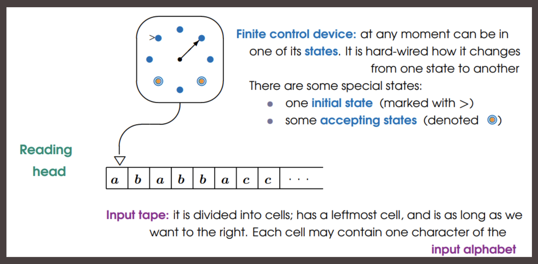
Finite Automata or Finite-State machines
A theoretical model for programs that use a constant amount of memory regardless of the input form
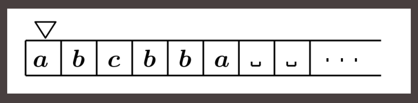
Finite automaton: how it starts
- The finite control devices is in its unique initial state
- The tape contains a finite word of the input alphabet, the input, as its left end. The remainder of the tape contains only blank cells
- The reading head is positioned on the leftmost cell of the input tape, containing the first character of the input word
Finite automation: how it works
- At regular time intervals, the automaton:
- reads one character from the input tape
- moves the reading head one cell to the right
- changes the state of its control device.
- The control devices is hard-wired so that the next state depends on:
- the previous state
- the character read from the tape.
- As the input is finite, at some moment, the reading head reaches the end of the input word (that is, the first black cell)
- If, at this moment, the control device is in one fo the accepting states, then the input word is accepted by the automaton. Otherwise, the input word is not accepted (or rejected)
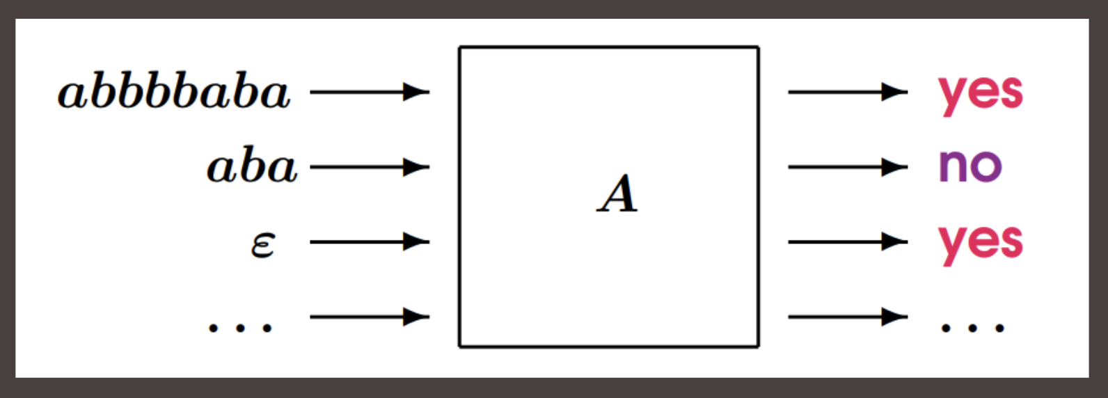
Finite automaton: what they are used for
- Each finite automaton is a kind of “recognition” or “decision” device over all possible words of its input alphabet
- Each automaton can be “tried” on infinitely many input words, and gives a yes/no answer each time
- The set of words in the input alphabet that are accepted by the automaton is called the language of this automaton
abbbbaba -> |-----------| -> YES
     aba -> | Automaton | -> NO
     e   -> |           | -> YES
     ... -> |-----------| -> ...
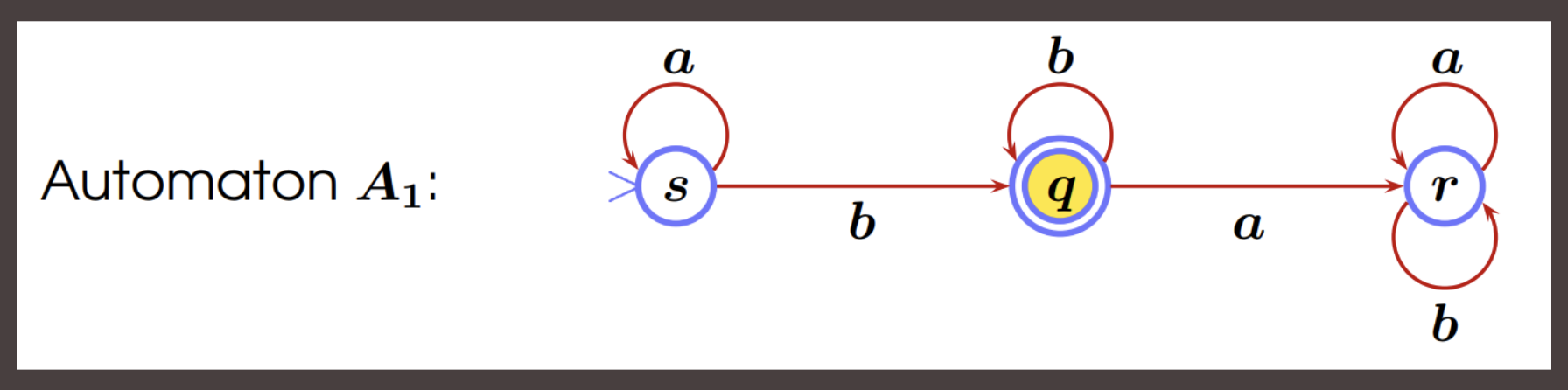
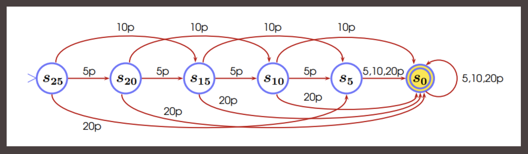
Lecture 3: Finite state machines and languages #
(内容省略)
Week 7: Data structures: representations and operations #
キーコンセプト
This topic includes:
- notation and terminology for data structures and algorithms,
- stacks
- queues
- deques
- operations on lists.
レクチャーリスト
- Introduction to data structures and algorithms
- Lecture 1: General introduction to sequences, terminology and notation
- Linear lists and operations
- Lecture 2: Linear lists – stack, queue, deque. Insertion and deletion
- Programming operations on lists in Python
- Lecture 3: Using linear data structures in Python
Lecture 1: General introduction to sequences, terminology and notation #
Data structures: representations and operations
- We consider the types of data structure best suited to particular operations on data, with regard to the efficiency of these operations and the effective use of storage
- We begin this topic with linear lists and sequences
- We will progress to cover trees, tree traversal, sorting and search
Linear list
- A linear list is a set of n nodes (where n >= 0) X[1], X[2], X[3] … X[n] whose structural properties essentially involve only the linear (one-dimensional) relative positions of the nodes.
- This includes the most popular and array data structures you might be familiar with from programming languages like Python or Java
Basic built-in Python sequence types: list, tuple ,str
- The principle of “encapsulation” in object-oriented design states that a programmer should not need to know the details of how a data structure or algorithm is implemented, only the “interface” to the structure; that is, how to use it
- However, hare we are concerned with how best to implement a sequence for good performance and memory efficiency, so we will look into these structures
- The primary memory of a computer is composed of bits of information, and those bits are typically grouped into larger units that depend upon the precise system architecture
- Such a typical unit is a byte, which is equivalent to 8 bits
- A computer system will have huge number of bytes of memory, and to keep track of what information is stored in what byte, the computer uses an abstraction known as a memory address
- In effect, each byte of memory is associated with a unique number that serves as its address
- Despite the sequential nature of the numbering system, computer hardware is designed, in theory, so that any byte of the main memory can be efficiently accessed based upon its memory address
- In this sense, wa way that a computer’s main memory performs a random access memory (RAM)
- A group of related variables can be stored one after another in a contiguous portion of the computer’s memory. We will denote such a representation as an array.
Linear lists (sequences) in Python
- In Python, each character is represented using the Unicode character set and, on most computing systems, Python internally represents each Unicode character with 16 bits (i.e. 2 bytes)
- Therefore, a six-character string, such as “SAMPLE”, would be stored in 12 consecutive bytes of memory
- We call each location in the array a “cell”, and its position its “index”
- The character P is at index 3 below
- Each cell uses the same number of bytes
- Therefore, a cell in an array can be accessed directly using only the memory address of the beginning of the array, the cell size and the index
start + (cellsize * index)
#address #4288 #4289 #4290 #4291 #4292 #4293 #4294
data...  S     A     M     P     L     E     data...
- In practice, we often want to store variable length records at each position of the array (i.e. not just a 16-bit string)
- Therefore, a referential list stores “references” (memory addresses) that refer to where the record is in memory
- These references are fixed-length memory address
- Arrays, like the one on the previous slide, where the data is stored directly rather than through a references, are “compact” arrays: those have fewer overhead memory costs than referential structures
#address #4288 #4289 #4290 #4291 #4292 #4293 #4294
data...  #ref0 #ref1 #ref2 #ref3 #ref4 #ref5 data...
- Python str is a compact array for storing characters sequentially
- Python lists and tuples are referential arrays
- str, list and tuple have constant time access
Lecture 2: Linear lists – stack, queue, deque. Insertion and deletion #
Stack
- A stack is a collection of objects that are inserted and removed according to the last-in, first-out (LIFT) principle. (Or, “push-down list”, “nesting store”). Push and Pop.
- All deletions and insertions (and usually accesses) occur at one end of the list, known as the top
- e.g.,
- A web browser stores the addresses of recently visited sites in a stack. Each time a user visits a new site, that site’s address is pushed onto the stack of addresses. The browser then allows the user to pop back to previously visited sites using the back button
- When a running computer program calls a function, the address of the place to return to when the function finishes is pushed onto the call stack. If that function calls another function, its return address is pushed onto the call stack. When a function completes, the return address is popped from the stack
Queue
- A queue is a collection of objects that are inserted and removed according to the first-in, first-out (FIFO) principle. Enqueue and Dequeue.
- All deletions (and usually accesses) occur at one end called the “front:, and all insertions at the other end called the “rear” of the list
- e.g.,
- A server responding to requests
- A ticketing system receiving and processing orders
- A call centre taking incoming calls
Double-ended queue
- A deque (pronounced “deck”) or double-ended queue is a collection where deletions and insertions (and usually accesses) occur only at the left and right ends of the list
- Therefore, the deque has operations like add_left, delete_left and add_right, delete_right insert and remove nodes. These could also be named add_first, add_last etc.
Linked list
- An alternative to the array-based list structure that we saw in the first lesson in this topic is the liked list
- Each node in a linked list stores some data and a reference (a link) to the next node
- The first and last nodes of the linked list are known as the head and tail of the list
- We traverse the list by starting at the head and, following the references, hopping along the links
Array-based vs link-based structures
- Advantages of array-based (sequential allocation) structures
- Arrays provide constant time access to an element based on an integer index and better caching behaviour.
- Link-based structures require extra memory overhead to store hte references (although have better memory usage in some cases) but easier insertion and deletion at any point in the list, easy concatenation, splitting and resizing of the list
Lecture 3: Using linear data structures in Python #
(内容省略。Python を使って各データ型を自作クラスとして実装する例示。)
Further material #
- Data Structures: Stacks and Queues - YouTube
Week 8: Trees, forests, binary trees #
キーコンセプト
This topic includes:
- trees
- forests
- binary trees
- tree traversal.
レクチャーリスト
- Trees and forests
- Lecture 1: Definitions of trees: nodes, branches, leaves, levels; binary trees
- Binary trees
- Lecture 2: Definitions and examples of binary trees
- Implementing trees in Python
- Lecture 3: Implementing trees with linked structures and arrays in Python
Lecture 1: Definitions of trees: nodes, branches, leaves, levels; binary trees #
Trees: hierarchical data structures
- In the previous topic, we learned about linear data structures
- In real-world applications, data is very often hierarchical
- We can represent hierarchical data using trees.
Trees: representation
- A tree data structure is typically visualised by placing nodes (elements) inside circles or rectangles and drawing lines connecting parents and children
- With the exception of the top element, every element has a parent
- We typically call the top element the root and draw the children below the parent nodes (the opposite to how we draw a botanical tree!)
Trees: further terminology
- Nodes that have no children are called external nodes or leaves
- Nodes within the tree that have children are called internal nodes
- Nodes that are children of the same parent are siblings
Lecture 2: Definitions and examples of binary trees #
(内容省略。Python を使って掲題の構造を自作クラスとして実装する例示。)
Lecture 3: Implementing trees with linked structures and arrays in Python #
(内容省略。Python を使って掲題の構造を自作クラスとして実装する例示。)
Further material #
- Tree (General Tree) - Data Structures & Algorithms Tutorials In Python #9 - YouTube
Week 9: Tree traversal and other operations; binary search trees #
キーコンセプト
This topic includes:
- tree traversal
- binary search trees
- tree traversal
- search tree implementation.
レクチャーリスト
- Traversing binary trees
- Lecture 1: Traversal orders for binary trees: pre-order, post-order, breadth-first, in-order
- Binary search trees
- Lecture 2: Binary search trees: motivation and definitions, operations on binary trees
- Operations on binary trees
- Lecture 3: Tree traversal and working with binary search trees in Python
Lecture 1: Traversal orders for binary trees: pre-order, post-order, breadth-first, in-order #
Tree traversal
- One of the most common operations we might want to perform on a tree is to visit (i.e. access) all of the nodes in the tree
- This is called a “traversal” of a tree
- Visiting all of the nodes of other linked structures, such as linked lists or graphs, is also called “traversal”
- There are different kinds of tree traversal, corresponding to different orders of visiting the nodes
- The different traversals are useful in different contexts for particular applications, such as printing nodes in a certain order or searching a game sate tree
Preorder traversal
- In a preorder traversal of a tree T, the root of T is visited first and then the subtrees rooted at its children are traversed recursively. If the tree is ordered, then the subtrees are traversed according to the order of the children.
Postorder traversal
- In a postorder traversal of a tree T, children of the root node are recursively traversed first, and then the root is visited.
Breadth-first traversal: nodes are visited in level-order
- is a graph or tree traversal algorithm that explores all nodes at the current depth level before moving on to the next level.
Inorder traversal
- In an inorder traversal of a tree T, left subtree of T is visited recursively first, then T itself, and then the righ subtree
- This really only makes sense for binary trees
Lecture 2: Binary search trees: motivation and definitions, operations on binary trees #
(内容省略)
Lecture 3: Tree traversal and working with binary search trees in Python #
(内容省略。Python を使って掲題の構造を自作クラスとして実装する例示。)
Further material #
- Data Structures: Trees - YouTube
Week 10: Sorting and searching #
キーコンセプト
This topic includes:
- insertion sort
- quick sort
- merge sort
- lower bounds
- sorting algorithm complexity
- built-in sorting in Python
レクチャーリスト
- Sorting arrays
- Lecture 1: Sorting and searching
- Divide and conquer sorting algorithms
- Lecture 2: Merge sort, quicksort, and algorithm analysis
- Sorting continued: implementations and examples
- Lecture 3: Python implementations of sorting and searching
- Python built-ins
- Lecture 4: Built-in sorting methods in Python
Lecture 1: Sorting and searching #
(内容省略。バイナリサーチについて。)
Lecture 2: Merge sort, quicksort, and algorithm analysis #
(内容省略。マージソートとクイックソートについて。)
Lecture 3: Python implementations of sorting and searching #
(内容省略。Python を使って掲題の構造を自作クラスとして実装する例示。)
Lecture 4: Built-in sorting methods in Python #
(内容省略。Python のビルドインメソッドの単なる紹介。)
Further material #
- Algorithms: Quicksort - YouTube
Week 11, 12 #
最終課題の期間。コースワークで学んだ内容に関する大問 10 個、全 50 問程度の問題集に回答して提出する。